Coherence

Coherence is a measure of similarity between waveforms or traces. SamiGeo offers the energy-ratio algorithm application for computation of coherence, which is a variation of the eigenstructure approach. The eigenstructure method is based on the eigenvectors and eigenvalues of the covariance matrix as was introduced by Gersztenkorn and Marfurt (1999). The covariance matrix is constructed from the analytic trace composed of the original data and its Hilbert transform along structural dip to prevent ‘structural leakage’ corresponding to zero crossings (Chopra and Marfurt, 2007). The eigenstructure coherence as proposed by Gersztenkorn and Marfurt (1999), is simply given as the ratio of the first (and by definition, the largest) eigenvalue to the trace of the matrix. The energy ratio coherence is a slightly more general computation in that it is taken as ratio of the energy of the weighted principal component filtered analytic traces, to the sum of the energy of the analytic traces or total energy.

Comparison of time slices (at 1333 ms) from (a) seismic and (b) coherence volumes. Notice the subtle channel signature is not clear on the seismic data. (Adapted from Chopra and Marfurt, 2012; Data courtesy: TGS, Calgary)

The images above show the comparison of equivalent time slices from a seismic and a coherence volume. Notice the clarity and detail that coherence provides in making the channels stand out.

As semblance is the commonly available algorithms available in workstation software packages, we depict below the comparison between the semblance and energy-ratio coherence.  Notice the sharp, crisp and more continuous definition of the lineaments seen on the energy-ratio display.

Comparison of stratal slice displays just above the Hunton Limestone marker through coherence volumes generated using (a) semblance, and (b) energy-ratio algorithms using analytic traces and the same 5-trace by 20-ms analysis window oriented along structural dip.  Green arrows indicate zones of improved fault continuity using energy-ratio coherence. Red arrows indicate zones of greater noise in the semblance coherence. Overall, the energy-ratio coherence slices exhibit crisper, more detailed lineaments than the semblance coherence for this geologic formation. (Adapted from Chopra and Marfurt (2018); Data courtesy: TGS, Houston)

Multispectral coherence

Coherence computed on specific voice component volumes exhibit more and crisp lineaments information than just the input seismic volume. Up to three voice component coherence volumes can be blended using the RGB color scheme, but if the coherence volumes to be blended becomes more than 3, then it becomes a limitation of the RGB blending.

Sui et al. (2015) addressed the multispectral coherence analysis problem by constructing a covariance matrix from the spectral magnitudes am:

where L is the number of spectral components. They found the resulting coherence images to be higher quality than that computed from the broad band data, including most of the details seen in coherence computed by constructing covariance matrices from the individual magnitude components. By ignoring the phase component, they also found that the algorithm was less sensitive to structural dip, resulting in algorithmic simplification.

Marfurt (2017) built on these ideas, but constructed a multispectral covariance matrix oriented along structural dip using the analytic voice components, and therefore twice as many sample vectors (i.e. spectral voices and their Hilbert transforms):

The corresponding energy ratio coherence computed using this equation is then referred to as multispectral coherence. We notice that multicoherence displays exhibit more focused and distinct lineament detail than the broadband seismic data.

Stratal slices 86 ms below a prominent marker at about 850 ms through the (a) broadband coherence, and (b) multispectral coherence volumes generated on seismic data acquired over the STACK trend in Oklahoma. Yellow block arrows indicate a channel more clearly on the multispectral coherence. Similarly, an offshoot channel is seen more clearly on multispectral coherence as indicated by the blue arrow. (Adapted from Chopra and Marfurt (2018); Data courtesy: TGS, Houston)

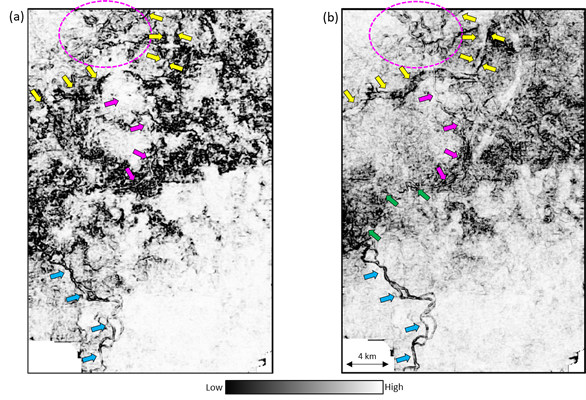
Stratal slices 160 ms below a prominent marker at about 850 ms through the (a) broadband coherence, (b) multispectral coherence volumes generated on seismic data acquired over the STACK trend in Oklahoma. Notice the better definition of the channel features as indicated by the yellow and magenta arrows as well as in the highlighted area. There is at least one channel feature running north-south as indicated by the blue, green, magenta arrows as well as the highlighted portion on top. (Adapted from Chopra and Marfurt (2018); Data courtesy: TGS, Houston

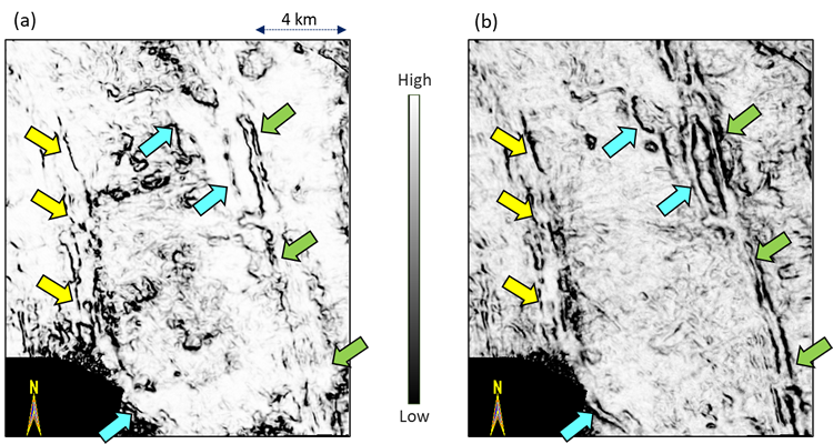
Stratal slices 36 ms above a marker at roughly 1700 ms through the (a) broadband coherence and (b) multispectral coherence volumes. Notice, the overall better definition of faults indicated with yellow, cyan and green arrows. The seismic data are from the Montney-Dawson area in British Columbia, Canada. (Adapted from Chopra and Marfurt (2018); Data courtesy: TGS, Calgary)

Multiazimuth coherence

With the focus on shale resource plays, wide azimuth surveys are being commonly acquired. Such surveys provide better quality data in terms of less coherent noise coming from ground roll, and interbed multiples, as well as azimuthal anisotropy analysis.  Coherence on azimuth-sectored data has been demonstrated before, and though it exhibits better lateral resolution, it is found to be noisy. Similar to multispectral coherence, the covariance matrix is modified to be the sum of the covariance matrices, each coming from an azimuthally limited volume, and then using the summed covariance matrix to compute the coherent energy (Qi et al, 2017). This computation is referred to as multiazimuth coherence.

We demonstrate the application of multiazimuth coherence on real seismic data in the examples below and show the added value they provide for interpretation of geologic features that is always being sought.

Stratal slices 12 ms above a horizon at approximately 1950 ms through coherence volumes computed from the six azimuthally limited partial stack amplitude volumes shown in Figure 5, from the full stack volume, and using a multiazimuth coherence algorithm. The definitions of the faults as well as the channels are seen much better on the multiazimuth coherence display. The seismic data are from the STACK trend in Oklahoma (Adapted from Chopra and Marfurt (2019); Data courtesy of TGS, Houston).

Stratal slices 22 ms below a horizon at approximately 1950 ms through coherence volumes computed from the six azimuthally limited partial stack amplitude volumes shown in Figure 10, from the full stack volume, and using a multiazimuth coherence algorithm. Again, the multiazimuth coherence display stands out much better than the other displays. The seismic data are from the STACK trend in Oklahoma (Adapted from Chopra and Marfurt (2019); Data courtesy of TGS, Houston)

Stratal slices 12 ms above a horizon at approximately 1950 ms through coherence volumes computed from the four offset-limited partially stacked volumes, from the full stack volume, and using a multioffset coherence algorithm. The definition of the faults is clearer and more focused on the multioffset coherence display when compared with the other displays. The seismic data are from the STACK trend in Oklahoma (Adapted from Chopra and Marfurt (2019); Data courtesy of TGS, Houston).

References

• Chopra, S., and K. J. Marfurt, 2007, Seismic attributes for prospect identification and reservoir characterization, Geophysical Development Series, SEG.

• Gersztenkorn, A. and K. J. Marfurt, 1999, Eigenstructure-based coherence computations as an aid to 3D structural and stratigrahic mapping: Geophysics, 64, 1468-1479.

• Qi, J., F. Li, and K. J. Marfurt, 2017, Multiazimuth coherence, Geophysics, 82, no. 6, P083-089.

• Sui, J.-K., Zheng, X.-D. and Li, Y.-D., 2015, A seismic coherency method using spectral attributes. Applied Geophysics, 12, no. 3, 353-361.

• Marfurt, K. J., 2017, Interpretational aspects of multispectral coherence: 79th Annual EAGE Conference and Exposition, Expanded Abstract, Th A4 11.

• Chopra, S., and K. J. Marfurt, 2018, Multispectral coherence attribute applications, AAPG Explorer, July issue, 16.

• Chopra, S., and K. J. Marfurt, 2019, Multispectral, multiazimuth and multioffset coherence attribute applications, Interpretation, 7(2), SC21-SC32.

Curvature

Curvature refers to the degree of bending of a reflection surface and can be measured as the rate of change of the curved reflection in a given direction.  This would suggest that in the simplest way one could calculate curvature by computing the first and second derivatives of the x- and y- components of the surface. The surface computation of curvature involves fitting a quadratic surface to the mapped horizon using a least-squares regression and using nine sample points (eight neighbors around a given point). When nine sample points are used for the computation of curvature, it results in an overdetermined system when the solution is sought by the least squares regression method.  Different measures of curvature can then be written in terms of the six coefficients, as was shown by Roberts (2001).

For extension to volumetric computation of curvature, inline and crossline components of dip are computed, which Al-Dossary and Marfurt (2006) make use of to evaluate the derivatives numerically in the polynomial equation.

Of all the available curvature measures, Chopra and Marfurt (2007) recommend the application of the most-positive curvature and most-negative curvature attributes, for they are the easiest to understand intuitively.

Roberts (2001) ha given the following expression for computation of the most-positive curvature.

As we note above, curvature is a function of the first derivatives of the inline dip, p, and crossline dip, q.  In the method of Fourier filtering, Al-Dossary and Marfurt (2006) introduce a fractional index (α) based multispectral estimation of curvature. The derivative in  in the Fourier domain is equivalent to multiplying the spectrum by (ik), but Al-Dossary and Marfurt (2006) introduce a fractional index α such that the spectrum gets multiplied by it. The smaller values of α yield the long-wavelength estimates of curvature, and larger values the short wavelength.  The inverse Fourier transform allows the generation of 3D convolution operator, which is convolved with p and q to obtain filtered versions of  Both such estimates have their applications, long wavelength suitable for obtaining the gross definitions of the geometrical features and the short wavelength for extracting the finer details and thus more resolved images.

Stratal slices through (a) coherence, (b) most-positive curvature (long-wavelength), (c) most-positive curvature (short-wavelength), (e) most-negative curvature (long-wavelength), and (f) most-negative curvature (short-wavelength). Note the complementary image of faults and flexures generated from coherence and the short-wave curvature attributes, where the fault indicated by the yellow arrows loses offset it can no longer be seen in coherence but still exhibits curvature anomalies. (d) Co-rendered images of coherence and long wavelength curvature show that the strong incoherence anomalies indicating a rugose or highly faulted and fractured horizon (green arrows) are visually correlated to long wavelength synclines and anticlines which in turn measure areas of high strain. (Adapted from Chopra and Marfurt, (2015); Data courtesy: Arcis Seismic Solutions, TGS)

Euler curvature

Euler curvature is determined from the most-positive and most-negative curvature magnitudes as well as their strikes. Because the reflector dip magnitude and azimuth can vary considerably across a 3-D seismic survey, it is more useful to equally sample azimuths of Euler curvature on a horizontal x-y plane and project the lines onto the local dipping plane of the reflector. In this way, Euler curvature can be calculated in any desired azimuth across a 3-D seismic volume to enhance the definition of specific lineaments. Such enhanced lineaments along specific azimuths can be brought together for interpreting azimuth-dependent structure for convenient interpretation. We describe here the application of Euler curvature to a 3-D seismic volume from the Montney-Dawson area of northeastern British Columbia, Canada. The data volume displayed is close to 500 square kilometers.

Stratal display through a coherence volume at a level close to t=1600 milliseconds. Fault lineaments striking -30 degrees from north are indicated by red arrows. Another lineament striking approximately east-west is indicated by green arrows. (Adapted from Chopra and Marfurt, (2016); Data courtesy: Arcis Seismic Solutions, TGS)

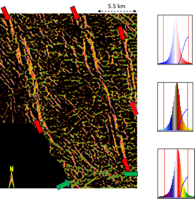
Stratal slices through long-wavelength Euler-curvature attribute volumes with strikes of: (a) ±90o, (b) -30o, and (c) +30o as indicated by the insets. In essence, Euler curvature is an azimuthally filtered version of the most-positive and most-negative principal curvatures, accentuating faults and flexures along any desired strike direction. The subtle lineaments seen in (c) may correspond to splay faults or relay ramps controlled by the major faults shown in (b). (Adapted from Chopra and Marfurt, (2016); Data courtesy: Arcis Seismic Solutions, TGS)

The same stratal slices shown in the previous figure, but now plotted against red, green, and blue color bars using opacity to enhance the most positive anticlinal features.  (Adapted from Chopra and Marfurt, (2016); Data courtesy: Arcis Seismic Solutions, TGS)

Co-rendering the three images of the anticlinal lineaments in the Figure above together using a modern 3D viewer and thus generating a composite display amenable to extracting more detailed interaction between the three hypothesized fault sets. (Adapted from Chopra and Marfurt, (2016); Data courtesy: Arcis Seismic Solutions, TGS)

References

• Roberts, A., 2001, Curvature attributes and their application to 3D interpreted horizons. First Break, 19, 85–99.

• Al-Dossary, S., and K. J. Marfurt, 2006, 3-D volumetric multispectral estimates of reflector curvature and rotation: Geophysics, 71, 41–51.

• Chopra, S., and K. J. Marfurt, 2007, Seismic attributes for prospect identification and reservoir characterization, Geophysical Development Series, SEG.

• Chopra, S. and Marfurt, K. J., 2015, Is curvature overrated? No it depends on the geology, First Break, 33 (2), 29-39.

• Chopra, S. and Marfurt, K. J., 2016, Interpreting fault and fracture lineaments with Euler curvature, AAPG Explorer, October issue, 22-23,25.