Elastic impedance inversion
As amplitudes of the near-offset traces are related to the changes in acoustic impedance they can be calibrated with well log curves or synthetic seismograms. However, if a far-offset or a far-angle stack has to be calibrated with the log data or synthetic seismograms, there is no analogous set of log curves that could be used for the purpose.
Back in 1999, Patrick Connolly from BP pointed this out and suggested the generalization of acoustic impedance for variable incidence angle using a linearized version of Zoeppritz equations. He called this elastic impedance and it provides the framework to calibrate and invert non-zero offset data. The elastic impedance approach is strongly dependent on the medium parameters (VP, VS, density and angle of incidence) and so is often regarded as the rock attribute analogue of acoustic impedance for varying angles of incidence.

Display of P-wave, S-wave, Density and Gamma-Ray log curves from a well in the Magdelena Valley, Colombia. The low values for all the curve displays are to the left and high values to the right. To the far right is shown a comparison of an AI curve with the computed EI(30°) curve. Notice the decrease in impedance (deviation in the blue and red curves) at the gas-producing zone as indicated with the purple arrow. (Adapted from Chopra and Sharma (2012); Data courtesy: PetroNorte, Colombia)

Synthetic seismogram tie for the low-angle (~10°) near-stack. The synthetic seismogram was generated by using the impedance log curve. The correlation seems to be reasonably good. (Adapted from Chopra and Sharma (2012); Data courtesy: PetroNorte, Colombia)

Synthetic seismogram tie for the high-angle (~30°) far-stack. The synthetic seismogram was generated by using the computed EI(30°) log curve. The correlation seems to be reasonably good. Notice the weakening of the amplitudes at the location of the orange arrows. (Adapted from Chopra and Sharma (2012); Data courtesy: PetroNorte, Colombia)
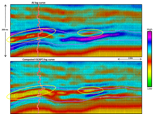
(Above) Segment of the acoustic impedance section (with the overlaid AI log) shows anomalously low values of impedance at the gas-producing zone (in yellow highlighted zone). (Below) Equivalent segment from EI(30o) section showing the anomaly as much more pronounced. (Adapted from Chopra and Sharma (2012); Data courtesy: PetroNorte, Colombia)
References
Chopra, S. and R. K. Sharma, 2012, An ‘Elastic Impedance’ Approach, AAPG Explorer, October issue, 40-41.