Extended elastic impedance inversion
Whitcombe et al., 2002 introduced extended elastic impedance (EEI), which broadened the definition of elastic impedance. According to this formulation, some of the rock properties cannot be predicted by the elastic impedance approach that usually considers the angle of incidence range as 0°–30°, which are the values taken by sin2θ. Consequently, by bringing about a change of variable, i.e., sin2θ replaced with tanχ, the angle range is extended from −90° to 90°, and this allows calculation of an impedance value beyond physically observable range of angle θ. The χ angle can be selected to optimize the correlation of the EEI curves with petrophysical reservoir parameters, such as Vclay, water saturation, and porosity or with elastic parameters such as bulk modulus, shear modulus, Lamé constants, and so on. It may be noted that χ is not the actual reflection angle, but it is an independent input variable that is required for computing EEI.

(a) Workflow for extended elastic impedance (EEI) approach for predicting the volume of petrophysical properties from seismic data. (b) Cross-correlation analysis for effective porosity (blue curve) and Vclay (green curve) with EEI curves. A maximum negative correlation is seen for effective porosity at 22°, and a maximum positive correlation is seen for Vclay at 28°.
We illustrate the different steps followed in the EEI approach in the figure (a) above. Because EEI reflectivities are crosscorrelated with desirable Vclay and effective porosity log curves for different values of the angles, the correlation coefficients are plotted in figure (b). The maximum positive correlation coefficient of 0.85 for Vclay (green curve) is seen at an angle of 28°, and a negative correlation coefficient of 0.9 at an angle of 22° (blue curve). The values of angles allow the determination of these properties (effective porosity and Vclay) from seismic data through the application of Zoeppritz equations on seismic angle gathers.
In figures (a) and (b) below, we exhibit equivalent crossline sections from the effective porosity and Vclay volumes with the respective petrophysical log curves overlaid on them. A reasonably good match between them is seen in both cases, which enhances our confidence in the application of the followed approach for the data at hand.

(a) A cross-line section from inverted effective porosity volume passing through a well. The overlaid effective porosity curve shows a strong correlation with inverted results. (b) Equivalent cross-line section from inverted Vclay volume passing through a well. The overlaid Vclay curve shows a strong correlation with inverted results. (Adapted from Chopra et al. (2017); Data courtesy: TGS, Asker)
Next, we crossplotted the effective porosity and Vclay derived attributes as shown in figure (a) below. On enclosing the cluster of points that exhibit high porosity and low values or not-so-low values of Vclay with red, green, and blue polygons, and back projecting on the vertical seismic, we are able to highlight these points coming from different zones.
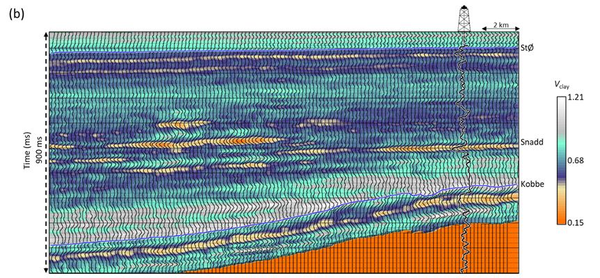
In figure (b), we see the differentiation of the potential reservoirs within the three formations of interest, namely, the Stø, Snadd, and Kobbe Formations. All these attribute volumes generated earlier, together with porosity and Vclay data volumes helped us generate displays at the levels of interest. This was a significant aid in studying the areal extent of the potential reservoirs present in the intervals of interest, which was the third objective for our exercise.

(a) Cross-plot of inverted effective porosity and Vclay volumes over the zone of interest (colour-coded with time). Cluster of points exhibiting high porosity and low Vclay values are enclosed by red, green and blue polygons. The back projection of these polygons on the seismic crossline is shown in (b). Notice, we are able now to differentiate the potential reservoirs within Stø , Snadd and Kobbe formations. (Adapted from Chopra et al. (2017); Data courtesy: TGS, Asker)
References
Chopra, S. and R. K. Sharma, 2012, An ‘Elastic Impedance’ Approach, AAPG Explorer, October issue, 40-41.
Chopra, S., R. K. Sharma, G. K. Grech, and B. E. Kjølhamar, 2017, Characterization of shallow high-amplitude seismic anomalies in the Hoop Fault Complex, Barents Sea, Interpretation, Vol. 5, No. 4 (November 2017); p. T607–T622.
Connolly, P., 1999, Elastic impedance: The Leading Edge, 18, 438–452, doi: 10.1190/1.1438307.
Whitcombe, D. N., P. A. Connolly, R. L. Reagan, and T. C. Redshaw, 2002, Extended elastic impedance for fluid and lithology prediction: Geophysics, 67, 63–67, doi: 10.1190/1.1451337.